Units#
Simulation and Physical Units#
Simulating gravitational systems often involves quantities spanning many orders of magnitude—parsecs, solar masses, gigayears. To ensure numerical stability, performance, and reproducibility, simulations are usually run in dimensionless “code units”, which must be chosen and handled with care. Odisseo makes no assumptions about your choice of units. Instead, it provides a flexible system for defining simulation units and converting between physical and code units.
⚠️ Why Unit Conversion Matters#
Numerical stability: Large or small values (e.g., 10⁻¹⁰ pc or 10¹⁰ \(M_\odot\)) can cause floating-point precision errors or instabilities during integration.
Physical meaning: Without clearly defined units, interpreting simulation results becomes error-prone.
Modularity: Whether you’re simulating a Milky Way analog or a dwarf galaxy, consistent unit handling makes your setup portable and interpretable.
Specify Simulation Units Explicitly#
When setting up a simulation in Odisseo, you must define your base units:
Unit of length (e.g., 1 kpc)
Unit of mass (e.g., 1e4 \(M_\odot\))
Optionally unit of time (e.g., 1 Myr), or a gravitational constant G in physical units (e.g., astropy.constants.G) The CodeUnits class will derive all other code units—such as time, velocity, and force—from your input, using Astropy units conversion in the backhend.
📌 Important: Every physical quantity you pass into the simulation (e.g., positions, masses, velocities) must be explicitly converted into code units using your
CodeUnitsinstance.
Example#
from astropy import units as u
from astropy import constants as c
from odisseo.units import CodeUnits #CodeUnits is a class with user defined astropy units
code_length = 10 * u.kpc #length simulation unit
code_mass = 1e4 * u.Msun #mass simulation unit
G = 1 #G here is just a place holder when time units are passed
code_time = 3 * u.Gyr #time simulation unit
code_units = CodeUnits(code_length, code_mass, G=1, unit_time = code_time ) #G and all the derived units are handled internally in the code_units object
### !! REMEMBER TO CONVERT YOUR PHYSICAL UNITS IN THE PARAMS AND CONFIG !!###
config = SimulationConfig(N_particles = 1000,
return_snapshots = True,
num_snapshots = 500,
num_timesteps = 1000,
external_accelerations=(NFW_POTENTIAL, MN_POTENTIAL, PSP_POTENTIAL),
acceleration_scheme = DIRECT_ACC_MATRIX,
softening = (0.1 * u.pc).to(code_units.code_length).value,) #CONVERSION TO SIMULATION UNITS
params = SimulationParams(t_end = (3 * u.Gyr).to(code_units.code_time).value,
Plummer_params= PlummerParams(Mtot=(10**4.05 * u.Msun).to(code_units.code_mass).value,
a=(8 * u.pc).to(code_units.code_length).value),
MN_params= MNParams(M = (68_193_902_782.346756 * u.Msun).to(code_units.code_mass).value,
a = (3.0 * u.kpc).to(code_units.code_length).value,
b = (0.280 * u.kpc).to(code_units.code_length).value),
NFW_params= NFWParams(Mvir=(4.3683325e11 * u.Msun).to(code_units.code_mass).value,
r_s= (16.0 * u.kpc).to(code_units.code_length).value,),
PSP_params= PSPParams(M = 4501365375.06545 * u.Msun.to(code_units.code_mass),
alpha = 1.8,
r_c = (1.9*u.kpc).to(code_units.code_length).value),
G=code_units.G, )
### RUN THE SIMULATION ###
snapshots = time_integration(initial_state_stream, mass, config, params)
### CONVERT BACK TO PHYSICAL UNITS ###
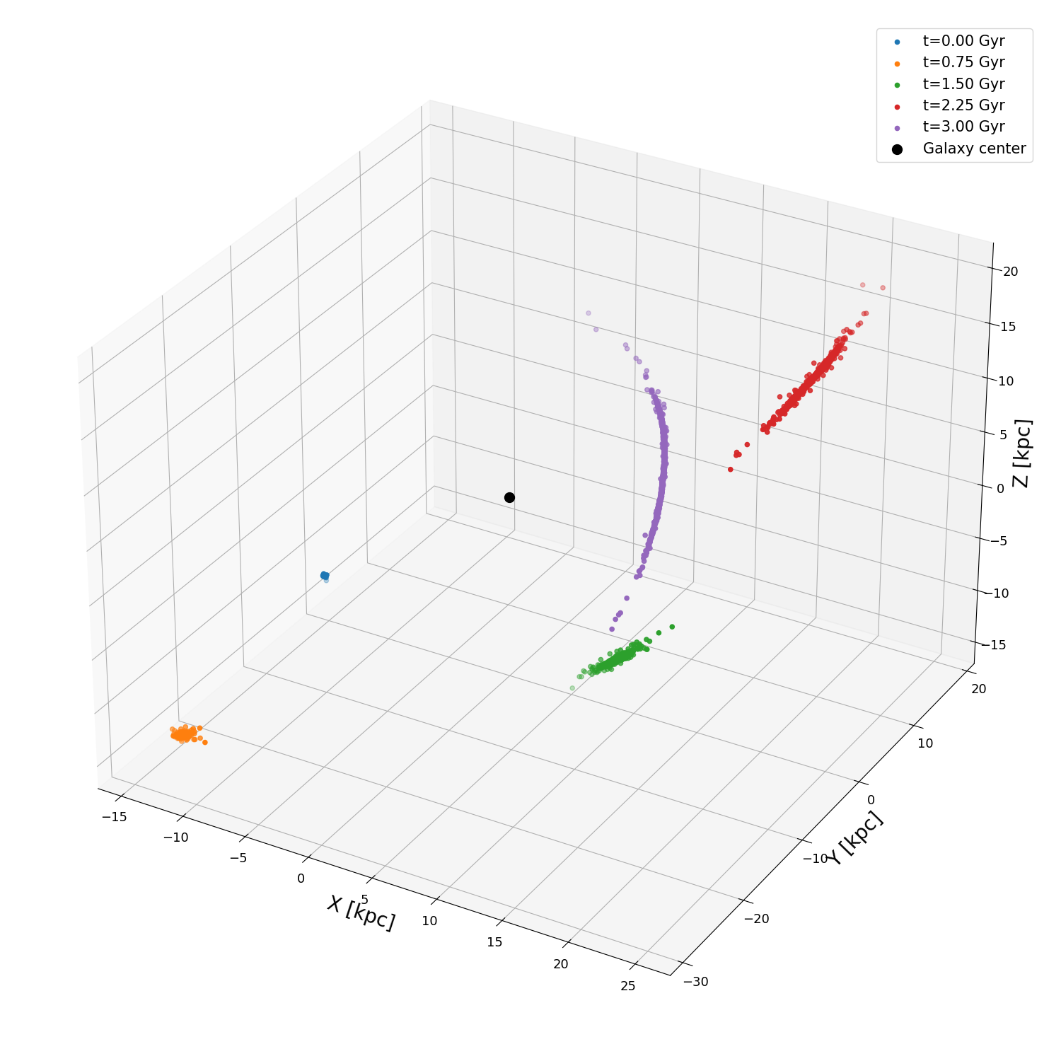
### here some snapshots positions are plotted
fig = plt.figure(figsize=(10, 10), tight_layout=True)
ax = fig.add_subplot(111, projection='3d')
for i in np.linspace(0, config.num_snapshots, 5, dtype=int):
ax.scatter(snapshots.states[i, :, 0, 0] * code_units.code_length.to(u.kpc), #CONVERSION TO PHYSICAL UNITS
snapshots.states[i, :, 0, 1] * code_units.code_length.to(u.kpc),
snapshots.states[i, :, 0, 2] * code_units.code_length.to(u.kpc), label=f"t={(snapshots.times[i]*code_units.code_time).to(u.Gyr):.2f}")
ax.scatter(0, 0, 0, c='k', s=100, )
ax.set_xlabel('X [kpc]')
ax.set_ylabel('Y [kpc]')
ax.set_zlabel('Z [kpc]')
ax.legend()
An example of the previous function is shown below: